《啥是佩奇》之 Mathematica 版-海边捡点贝壳

此文档为旧博客搬运。——2020.05.11

前两天意外在电视上看了很火的短视频《啥是佩奇》，感觉还挺有意思，尤其是最后鼓风机版佩奇出场的时候，颇有点黑客精神的味道。于是我就在想可否用 Mathematica 也画一个佩奇。网上简单搜了下，有用 Python 模拟画板一笔一笔画的，有用 CSS 渲染的，也有用 Mathematica 画不同曲线组合合成。CSS 渲染还算有点好玩，用 Python 和 Mathematica 模拟画板就有侮辱代码的嫌疑了。然后不知怎的就联想到了 Wolfram|Alpha 的 person curves ，用一些很复杂的式子画出名人的轮廓图，于是问题就转变为寻找画佩奇轮廓的公式表达式。当然，首先确认了下 Wolfram|Alpha 上没有佩奇（Peppa Pig）的曲线。

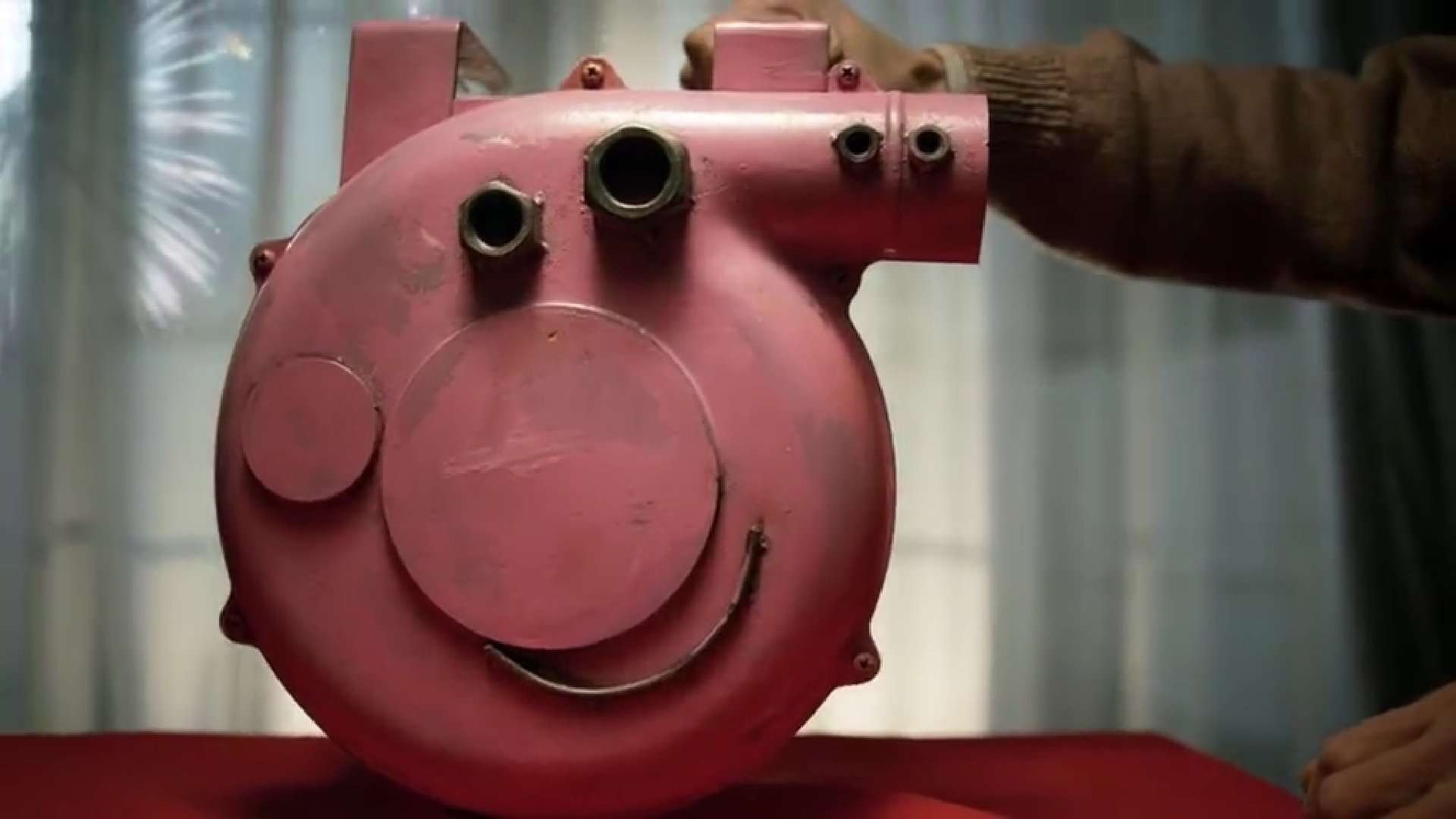Peppa Pig Snapshot 《啥是佩奇》中的“鼓风机版”佩奇

当然，轮子是不用再去造的——想来自己去造也不一定造得出来——官方博客也给出了用傅立叶级数近似的做法（见文末的第一个链接）。本文的代码几乎都来自该文，so, all credit goes to the author of the essay！

整个过程大概可分为三个部分：

图像轮廓识别；
寻找组成轮廓的曲线；
傅立叶近似各曲线。

图像轮廓识别

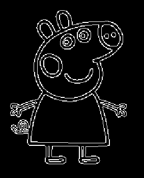
这里我稍微作弊了下，我选择的佩奇图像是一幅简单的素描：

peppapigsketch

在 Notebook 里面，让 peppaPigImage = 上面这幅图。

然后进行轮廓的探测：

peppaPigEdgeImage = EdgeDetect[peppaPigImage]

peppapigedge

再确定轮廓线上所有的点：

peppaPigEdgePoints = {#2, -#1} & @@@ 
   Position[ImageData[peppaPigEdgeImage], 1, {2}];

寻找组成轮廓的曲线

定义函数 pointListToLines，通过寻找随机点周边最近点的方式将这些点视为在同一条曲线上：

pointListToLines[pointList_, neighborhoodSize_: 6] := 
 Module[{L = DeleteDuplicates[pointList], NF, \[Lambda], lineBag, 
   counter, seenQ, sLB, nearest,  
               nearest1, nextPoint, 
   couldReverseQ,  \[ScriptD], \[ScriptN], \[ScriptS]},
  NF = Nearest[L] ;
       \[Lambda] = Length[L];
  Monitor[
   (* list of segments *)
   lineBag = {};
   counter = 0; 
   While[counter < \[Lambda],
    (* new segment *)
    sLB = {RandomChoice[DeleteCases[L, _?seenQ]]}; 
    seenQ[sLB[[1]]] = True;
    counter++;
    couldReverseQ = True;
    (* complete segment *)
    While[(nearest = NF[Last[sLB], {Infinity, neighborhoodSize}];
                 
      nearest1 = 
       SortBy[DeleteCases[nearest, _?seenQ], 
        1. EuclideanDistance[Last[sLB], #] &];
                 nearest1 =!= {} || couldReverseQ),
                  If[nearest1 === {},
                   (* extend the other end; penalize sharp edges *)
                   sLB = Reverse[sLB]; couldReverseQ = False,
                  (* prefer straight continuation *)
                   nextPoint = If[Length[sLB] <= 3, nearest1[[1]],
                                                 \[ScriptD] = 
         1. Normalize[(sLB[[-1]] - sLB[[-2]]) + 
            1/2 (sLB[[-2]] - sLB[[-3]])];
                                                 \[ScriptN] = {-1, 
           1} Reverse[\[ScriptD]];
                                                \[ScriptS] = 
         Sort[{Sqrt[(\[ScriptD].(# - sLB[[-1]]))^2 + 
                                                                      \
    (* perpendicular *) 2 (\[ScriptN].(# - sLB[[-1]]))^2], # } & /@ 
           nearest1]; 
                                                \[ScriptS][[1, 2]]];
                   AppendTo[sLB, nextPoint];
                  seenQ[nextPoint] = True;
                 counter++ ]];
    AppendTo[lineBag, sLB]];
   (* return segments sorted by length *)
   Reverse[SortBy[Select[lineBag , Length[#] > 12 &], Length]],
   (* monitor progress *)
   Grid[{{Text[Style["progress point joining", Darker[Green, 0.66]]], 
      ProgressIndicator[counter/\[Lambda]]},
               {Text[
       Style["number of segments", Darker[Green, 0.66]]],  
      Length[lineBag] + 1}}, 
            Alignment -> Left, Dividers -> Center]]]

这里，上述轮廓点可组成 15 条曲线：

SeedRandom[2];
hLines = pointListToLines[peppaPigEdgePoints, 5];
Length[hLines]
(*15*)

通过随机上色可以查看下这 15 条曲线的情况：

Graphics[{ColorData["DarkRainbow"][RandomReal[]], Line[#]} &  /@ 
  hLines]

peppapigrandomcolor

傅立叶近似各曲线

针对各曲线，通过 BSpline 近似，然后寻找其傅立叶级数的系数：

(* Fourier coefficients of a single curve *)
fourierComponentData[pointList_, nMax_, op_] := 
 Module[{\[CurlyEpsilon] = 10^-3, \[Mu] = 2^14, M = 10000, s,
                scale, \[CapitalDelta], L , nds, sMax, 
   if, \[ScriptX]\[ScriptY]Function, X, Y, XFT, YFT, type},
  (* prepare curve *)
  scale = 
   1. Mean[Table[ 
      Max[ fl /@ pointList] - 
       Min[fl /@ pointList], {fl, {First, Last}}]];
   \[CapitalDelta] = 
   EuclideanDistance[First[pointList], Last[pointList]];
   L = Which[op === "Closed", type = "Closed";
                                                            
    If[First[pointList] === Last[pointList], 
                                                                
     pointList, Append[pointList, First[pointList]]], 
                    op === "Open", type = "Open"; pointList,
                     \[CapitalDelta] == 0., type = "Closed";  
    pointList,
                     \[CapitalDelta]/scale < op, type = "Closed"; 
    Append[pointList, First[pointList]],
                    True,  type = "Open"; 
    Join[pointList, Rest[Reverse[pointList]]]];
  (* re-parametrize curve by arclength *)
  \[ScriptX]\[ScriptY]Function = BSplineFunction[L, SplineDegree -> 4];
  nds = NDSolve[{s'[t] == 
      Sqrt[\[ScriptX]\[ScriptY]Function'[
         t].\[ScriptX]\[ScriptY]Function'[t]], s[0] == 0}, s, 
                              {t, 0, 1}, MaxSteps -> 10^5, 
    PrecisionGoal -> 4];
  (* total curve length *)
       sMax = s[1] /. nds[[1]];
       if = 
   Interpolation[
    Table[{s[\[Sigma]] /. nds[[1]], \[Sigma]}, {\[Sigma], 0, 1, 1/M}]];
  X[t_Real] :=  
   BSplineFunction[L][Max[Min[1, if[(t + Pi)/(2 Pi) sMax]] , 0]][[1]];
  Y[t_Real] :=  
   BSplineFunction[L][Max[Min[1, if[(t + Pi)/(2 Pi) sMax]] , 0]][[2]]; 
  (* extract Fourier coefficients *)
  {XFT, YFT} = 
   Fourier[Table[#[N @ t], {t, -Pi + \[CurlyEpsilon], 
        Pi - \[CurlyEpsilon], (2 Pi - 
           2 \[CurlyEpsilon])/\[Mu]}]] & /@ {X, Y};   
  {type, 2 Pi/Sqrt[\[Mu]] *
    ((Transpose[
         Table[{Re[#], Im[#]} &[Exp[I k Pi]  #[[k + 1]]], {k, 0, 
           nMax}]] & /@ {XFT, YFT}))}  ]

Options[fourierComponents] = {"MaxOrder" -> 180, "OpenClose" -> 0.025};

fourierComponents[pointLists_, OptionsPattern[]] := 
 Monitor[Table[
    fourierComponentData[pointLists[[k]],                           
                                                                      \
     If[Head[#] === List, #[[k]], #] &[ OptionValue["MaxOrder"]],
                                                                      \
     If[Head[#] === List, #[[k]], #] &[ OptionValue["OpenClose"]]],
                             {k, Length[pointLists]}],
   Grid[{{Text[
       Style["progress calculating Fourier coefficients", 
        Darker[Green, 0.66]]], 
      ProgressIndicator[k/Length[pointLists]]} }, 
            Alignment -> Left, Dividers -> Center]] /; 
  Depth[pointLists] === 4

fCs = fourierComponents[hLines];

确定傅立叶级数：

makeFourierSeries[{"Closed" | "Open", {{cax_, sax_}, {cay_, say_}}}, 
  t_, n_] :=
  {Sum[If[k == 0, 1/2, 1] cax[[k + 1]] Cos[k t] + 
    sax[[k + 1]] Sin[k t], {k, 0, Min[n, Length[cax]]}],
   Sum[If[k == 0, 1/2, 1] cay[[k + 1]] Cos[k t] + 
    say[[k + 1]] Sin[k t], {k, 0, Min[n, Length[cay]]}]}

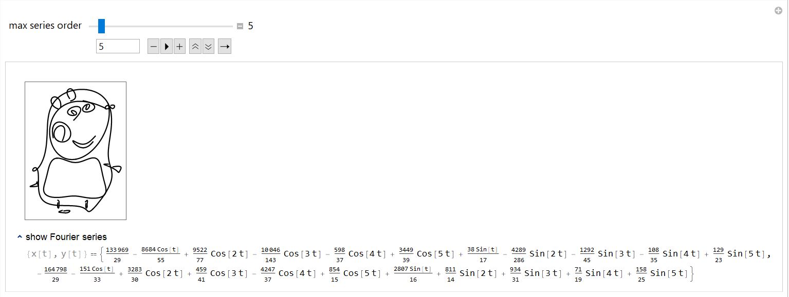
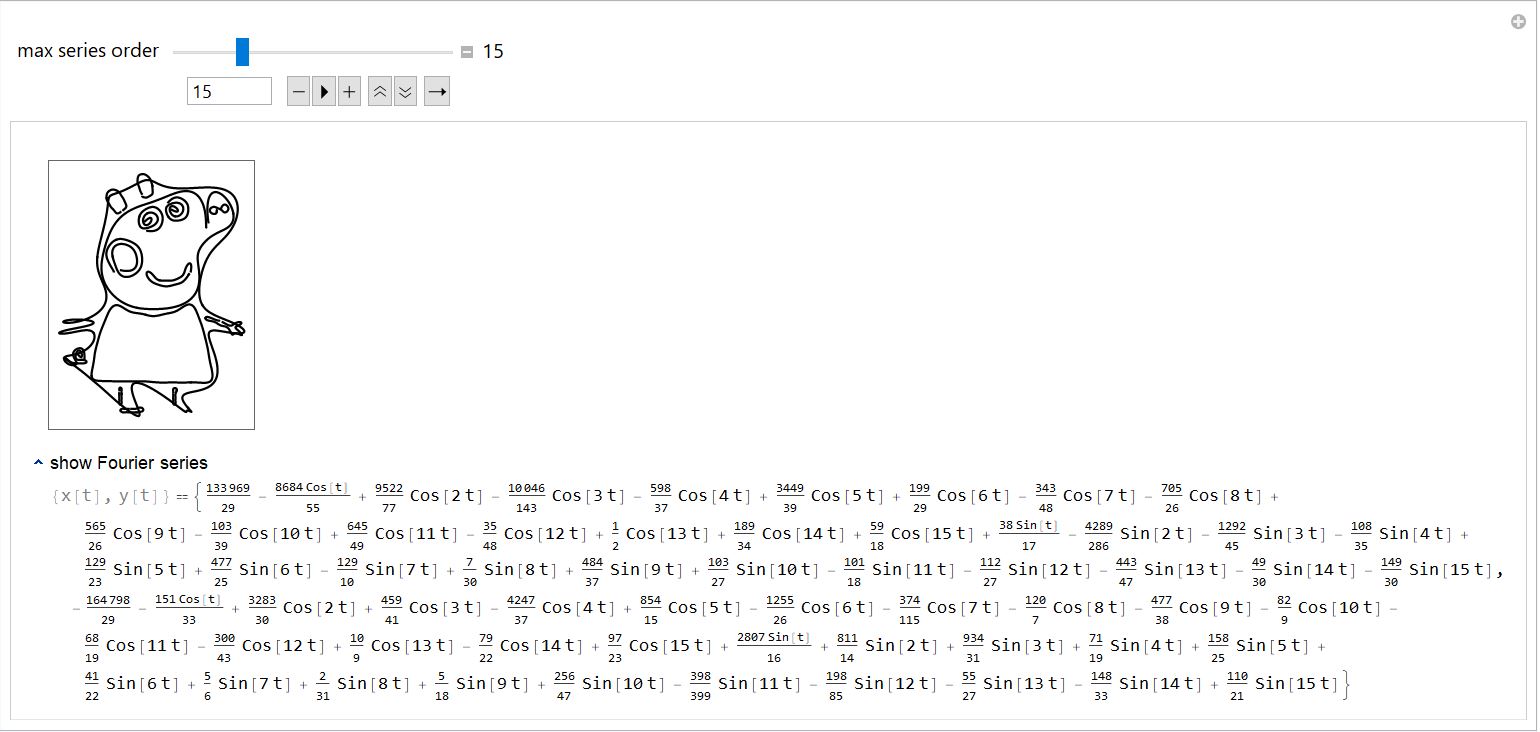
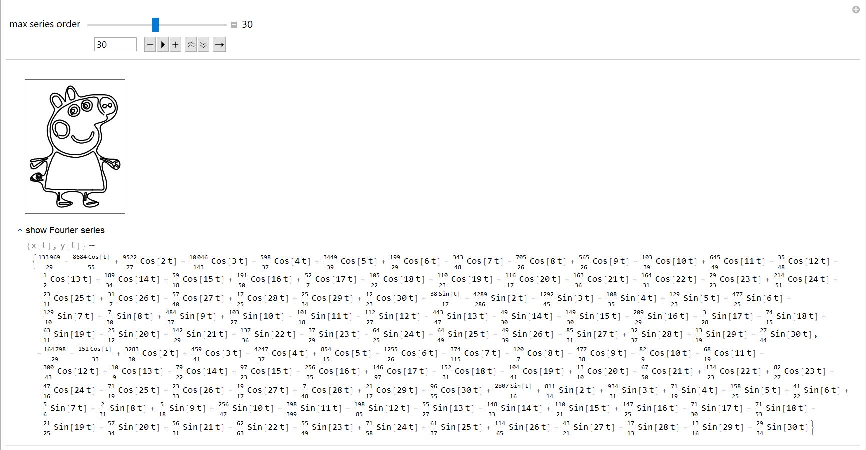
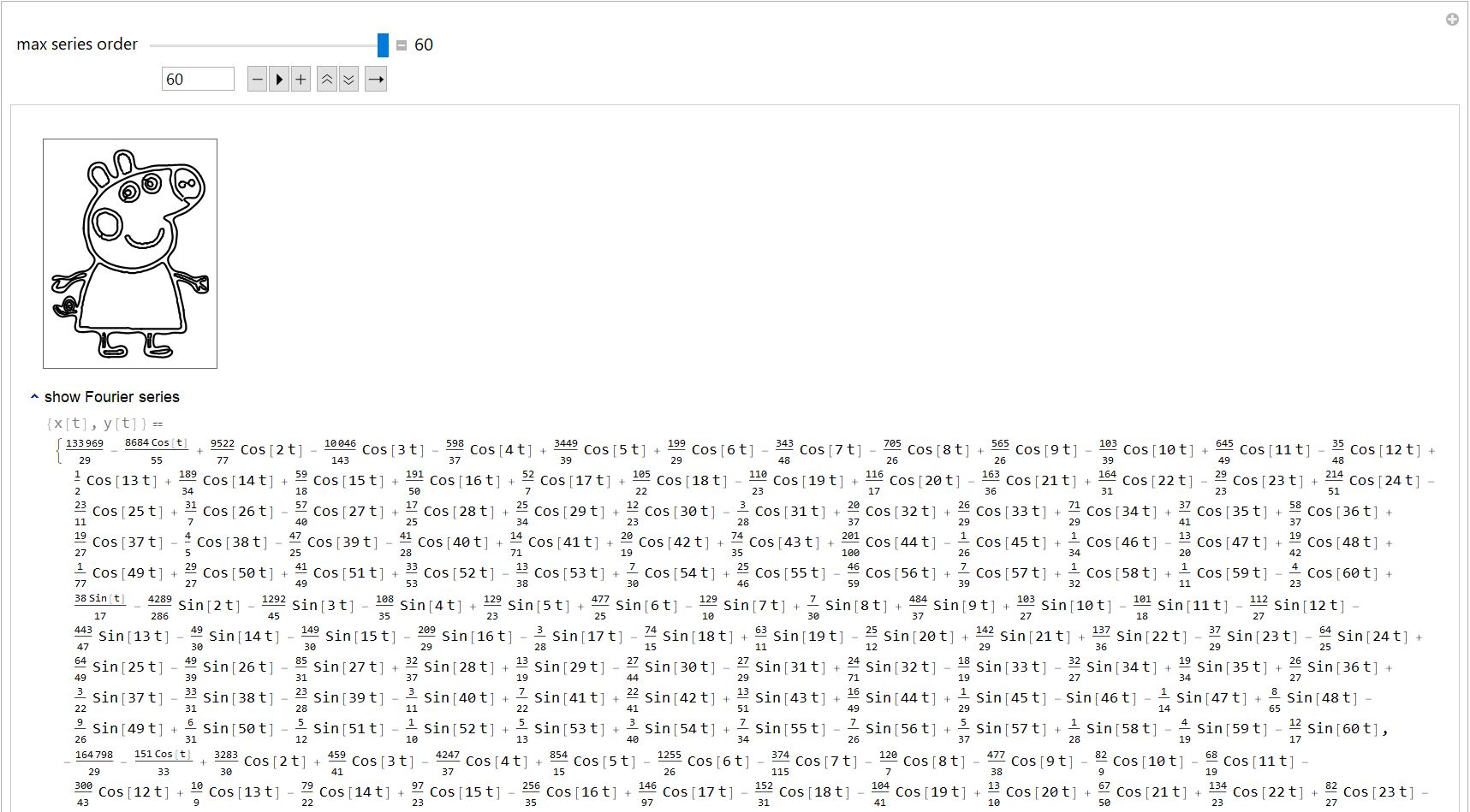
查看不同阶数近似的佩奇图及其傅立叶表达式（这里我简单修改了下，让其显示相应的傅立叶级数）:

makeFourierSeriesApproximationManipulate[fCs_, maxOrder_: 60] :=
 Manipulate[
  With[{opts = 
     Sequence[PlotStyle -> Black, Frame -> True, Axes -> False, 
                                               FrameTicks -> None, 
      PlotRange -> All, ImagePadding -> 12]},
   Column[
    {Show[{
        ParametricPlot[
         Evaluate[ 
          makeFourierSeries[#, t, n] & /@ 
           Cases[fCs, {"Closed", _}]], {t, -Pi, Pi}, opts],
        ParametricPlot[
         Evaluate[ 
          makeFourierSeries[#, t, n] & /@ 
           Cases[fCs, {"Open", _}]], {t, -Pi, 0}, opts]}] // Quiet,
     OpenerView[{Text["show Fourier series"], 
       Row[{Style[{x[t], y[t]}, Gray], 
         "\[ThinSpace]\[Equal]\[ThinSpace]", 
         Rationalize[(makeFourierSeries[#, t, n] & /@ fCs) // Total, 
          10^-3]}]}]
     }
    ]
   ], 
  {{n, 1, "max series order"}, 1, maxOrder, 1, 
   Appearance -> "Labeled"},
  TrackedSymbols :> True, SaveDefinitions -> True]

makeFourierSeriesApproximationManipulate[fCs]

可以得到不同阶数近似的佩奇：

peppapigorder5 peppapigorder15 peppapigorder30 peppapigorder60

其他

当然，这个也不仅仅 just for fun，事实上在用离散元（Discrete Element Method）模拟砂颗粒时，砂粒的不规则形状就可以通过傅立叶级数近似给出，而参考文中提到的其他方法也是值得研究的：

Fourier series are not the only way to encode curves. We could use wavelet bases or splines, or encode the curves piecewise through circle segments. Or, with enough patience, using the universality of the Riemann zeta function, we could search for any shape in the critical strip. (Yes, any possible [sufficiently smooth] image, such as Jesus on a toast, appears somewhere in the image of the Riemann zeta function ζ(s) in the strip 0 ≤ Re(s) ≤ 1, but we don’t have a constructive way to search for it.)

《啥是佩奇》之 Mathematica 版

目录

图像轮廓识别

寻找组成轮廓的曲线

傅立叶近似各曲线

其他

更多