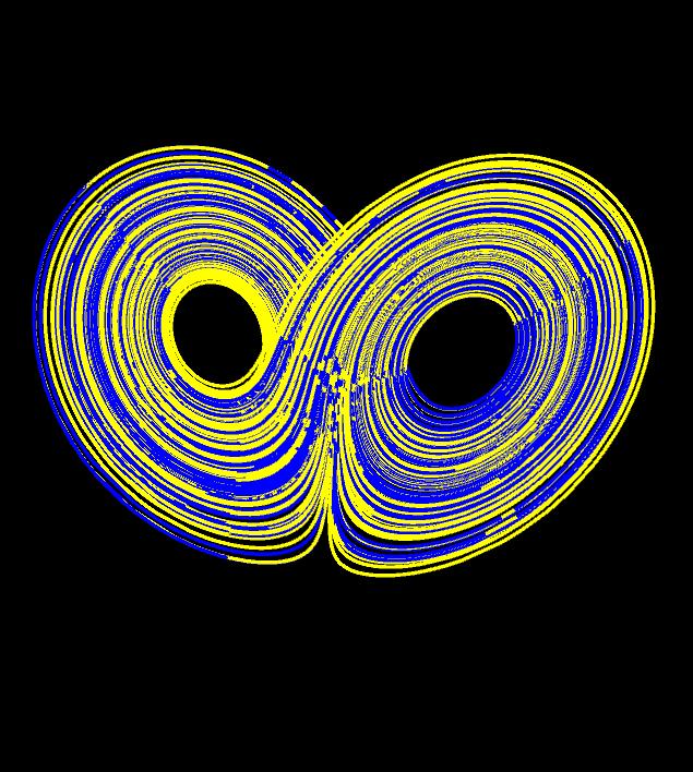
Mathematica plot of Lorenz system
此文档为旧博客搬运。——2020.05.11
Lorenz system is a simplified mathematical model to describe the atmospheric convection. The system consists of three ordinary differential equations given as:
\[\begin{aligned} \dfrac{\mathrm{d}x}{\mathrm{d}t} &= \sigma (y-x) \\\\ \dfrac{\mathrm{d}y}{\mathrm{d}t} &= x(\rho-z)-y \\\\ \dfrac{\mathrm{d}z}{\mathrm{d}t} &= xy -\beta z \end{aligned}\]where $x$, $y$ and $z$ are the system state, $t$ is time, and $\sigma$, $\rho$, $\beta$ are the system parameters.
The above ODE system can be solved by the following code in Mathematica:
tend = 100;
eq = {x'[t] == \[Sigma] (y[t] - x[t]),
   y'[t] == x[t] (\[Rho] - z[t]) - y[t],
   z'[t] == x[t] y[t] - \[Beta] z[t]};
init1 = {x[0] == 10, y[0] == 10, z[0] == 10};
init2 = {x[0] == 10, y[0] == 10, z[0] == 10.1};
pars = {\[Sigma] -> 10, \[Rho] -> 28, \[Beta] -> 8/3};
{xs1, ys1, zs1} =
  NDSolveValue[{eq /. pars, init1}, {x, y, z}, {t, 0, tend}];
{xs2, ys2, zs2} =
  NDSolveValue[{eq /. pars, init2}, {x, y, z}, {t, 0, tend}];
ParametricPlot3D[{{xs1[t], ys1[t], zs1[t]}, {xs2[t], ys2[t],
   zs2[t]}}, {t, 0, tend}, PlotStyle -> {Red, Blue},
 PlotPoints -> {1000, 1000}, Boxed -> False, Axes -> False]
A beautiful (well, the rendering color is not…) butterfly is traced out by the above code:

For further description of the system and code, please refer to https://en.wikipedia.org/wiki/Lorenz_system
Related reading
- Chaos: http://www.chaos-math.org/en